The problem with 3D blue noise
Update 2017-02-10: The normalization of the discrete Fourier transform has been changed to make it unitary and a note on the Fourier slice theorem has been added as suggested by Won Chun in the comments.
After the previous blog post several readers (namely Morgan McGuire, Mikkel Gjoel and Bart Wronski) expressed interest in 3D blue noise. Thus, this blog post provides a database of such blue noise textures. It also explains why you might not want to use it. The post relies on concepts introduced in the previous post so you should read this one first.
The implementation of the void-and-cluster method [Ulichney93] naturally generalizes to blue noise textures with arbitrary dimensions because the underlying operations (Gaussian blur and finding darkest pixels) do. Therefore, the generation of 3D blue noise is not much of a problem. Only the run time can grow intractable because it is \(O(n^2\cdot\log(n))\) where \(n\) is the number of output values (e.g. pixels or voxels).
Dithering seems like a good reason to consider 3D blue noise. With 2D blue noise textures we argue that the human visual system blurs everything slightly in the spatial domain, so the high-frequent noise introduced by blue noise dithering is hardly noticeable. Beyond that, the eye may be a little slow to recognize change at high frame rates such that it effectively also blurs in the temporal domain. If we use subsequent slices from a 3D blue noise texture in subsequent frames, we should be able to benefit from this. Exploiting this additional dimension might let us outperform independently computed 2D blue noise textures.
If this argument sounds fishy to you, you are right. It does not work that way but learning why is interesting and will be the main topic of this blog post. With that said, there are still some valid applications for 3D blue noise that we also look into.
Good 3D blue noise is bad 2D blue noise
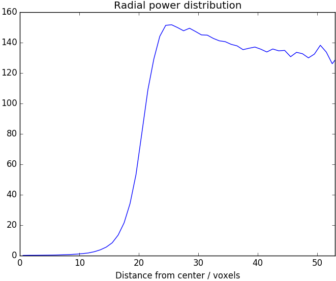
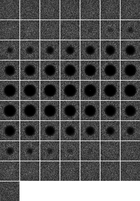
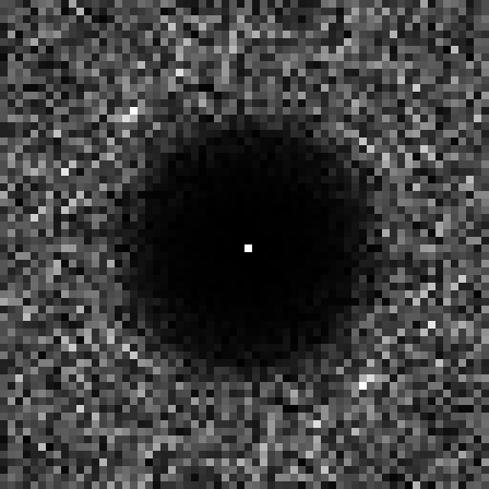
For the upcoming examples we consider a 3D blue noise texture with a total of 64³ voxels. It is the result of GetVoidAndClusterBlueNoise((64,64,64),1.9). As for 2D blue noise, it is useful to look at the distribution of energy in radial frequency bands. We expect weak low-frequency components and strong high-frequency components. Figure 1 shows that this is exactly what we get. The 3D Fourier transform has a spheric region with small values in the center and fairly uniform frequency content elsewhere as shown in Figure 2. From this figure it is also apparent that the blue noise is isotropic. By construction the 3D blue noise texture is also tileable and it contains each value from 0 to 64³-1 exactly once, so it is perfectly uniform.
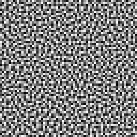
In summary, this is good 3D blue noise. All the properties that we like to see in 2D blue noise carry over analogously. So let's take a closer look at the 3D blue noise texture itself. Of course we cannot look at the whole 3D volume at once. Instead we consider the 2D slice from the 3D volume shown in Figure 3. This is where things turn bad. It does not really look like 2D blue noise. There are obvious brighter and darker regions. For comparison Figure 4 shows a 64² 2D blue noise texture which lacks these large-scale structures.

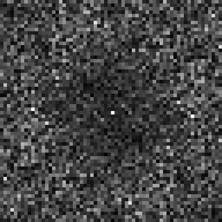
This is not mere appearance. We can consider the Fourier transform of the 2D slice from the 3D blue noise texture, which is shown in Figure 5. The low-frequency components in the middle are slightly weaker than the high-frequency components but much stronger than they should be for 2D blue noise. Figure 6 shows the Fourier transform for the 64² 2D blue noise texture. This is what we would like to have.
A first intuitive explanation is that 3D blue noise does not really enforce 2D blue noise properties for its slices. What 3D blue noise enforces is that application of a 3D blur makes the 3D texture nearly uniform. One way to accomplish this is by having a cluster of bright voxels in one slice next to a cluster of dark voxels in the adjacent slice. This means that clusters of similar values within 2D slices are possible but for 2D blue noise this is exactly what we want to avoid.
We can also look at it in a more rigorous fashion but it will require a slightly advanced use of signal processing theory. Taking a single slice out of the 3D volume is essentially the same as multiplying everything except for this slice by zero. By the convolution theorem, this multiplication in the spatial domain corresponds to a convolution in the frequency domain. The signal that we convolve with is the Fourier transform of what we multiplied by. If the slice that we keep is the one at index zero, this convolution happens to be a summation filter along the third dimension. So what really happens is that we sum the Fourier transform along the third dimension to get our 2D Fourier transform for the slice.
Admittedly, this explanation is still a little handwavy but if you are into signal processing, it probably helps to get across the basic idea of the proof. Another path to the same result is the Fourier slice theorem. If you still doubt the result, here is a self-contained proof.
Proposition: Let \(n_0,n_1,n_2\in\mathbb{N}\) be the dimensions of a 3D volume and let \(j\in\{0,\ldots,n_0-1\}\), \(k\in\{0,\ldots,n_1-1\}\) and \(l\in\{0,\ldots,n_2-1\}\) be corresponding indices. Let \(x(j,k,l)\in\mathbb{R}\) be a volume texture and let \(y(j,k):=x(j,k,0)\) be the first slice of this volume texture. Then the Fourier transforms \(\hat{x},\hat{y}\) of these signals are related by
\[\sqrt{n_{2}}\cdot\hat{y}(u,v)=\sum_{w=0}^{n_2-1}\hat{x}(u,v,w)\]where \(u\in\{0,\ldots,n_0-1\}\) and \(v\in\{0,\ldots,n_1-1\}\).
Proof: The proof relies on direct computation (and violation of the blog layout).
\begin{align} &\sum_{w=0}^{n_{2}-1}\hat{x}(u,v,w)\\ =&\frac{1}{\sqrt{n_{0}\cdot n_{1}\cdot n_{2}}}\cdot\sum_{w=0}^{n_{2}-1}\sum_{j=0}^{n_{0}-1}\sum_{k=0}^{n_{1}-1}\sum_{l=0}^{n_{2}-1}x(j,k,l)\cdot\exp\left(-2\cdot\pi\cdot i\cdot\left(\frac{u\cdot j}{n_{0}}+\frac{v\cdot k}{n_{1}}+\frac{w\cdot l}{n_{2}}\right)\right)\\ =&\frac{\sqrt{n_{2}}}{\sqrt{n_{0}\cdot n_{1}}}\cdot\sum_{j=0}^{n_{0}-1}\sum_{k=0}^{n_{1}-1}\sum_{l=0}^{n_{2}-1}x(j,k,l)\cdot\exp\left(-2\cdot\pi\cdot i\cdot\left(\frac{u\cdot j}{n_{0}}+\frac{v\cdot k}{n_{1}}\right)\right)\cdot\frac{1}{n_{2}}\cdot\sum_{w=0}^{n_{2}-1}\exp\left(-2\cdot\pi\cdot i\cdot\frac{l}{n_{2}}\right)^w\\ =&\frac{\sqrt{n_{2}}}{\sqrt{n_{0}\cdot n_{1}}}\cdot\sum_{j=0}^{n_{0}-1}\sum_{k=0}^{n_{1}-1}x(j,k,0)\cdot\exp\left(-2\cdot\pi\cdot i\cdot\left(\frac{u\cdot j}{n_{0}}+\frac{v\cdot k}{n_{1}}\right)\right)\\ =&\sqrt{n_{2}}\cdot\widehat{y}(u,v) \end{align}Note that we have applied the finite geometric series to conclude
\[\sum_{w=0}^{n_{2}-1}\exp\left(-2\cdot\pi\cdot i\cdot\frac{l}{n_{2}}\right)^w =\frac{1-\exp\left(-2\cdot\pi\cdot i\cdot l\cdot\frac{n_2}{n_{2}}\right)}{1-\exp\left(-2\cdot\pi\cdot i\cdot\frac{l}{n_{2}}\right)}=0\]for \(l\neq 0\). □
Now we know exactly why we have a problem. The Fourier transform of the 3D blue noise has a spherical region in the middle where frequency components are weak. However, if we sum it along the third dimension, we do not only sum over this region in the middle. The Fourier transform of 2D slices includes strong frequency content in low frequencies because the higher frequencies along the third dimension contribute to it. The 2D Fourier transform in Figure 5 is the sum of all the slices of the 3D Fourier transform shown in Figure 2.
Is there anything we can do about this? We do have a parameter that we could use for some tweaking, namely the standard deviation of the Gaussian filter used by the void-and-cluster-method. We can even use an anisotropic Gaussian. This effectively scales the sphere in the frequency domain where frequency content is weak. We can even take this to the limit with GetVoidAndClusterBlueNoise((64,64,64),(1.9,1.9,0.0)). The sphere is stretched out infinitely and degenerates into a cylinder as shown in Figure 7.
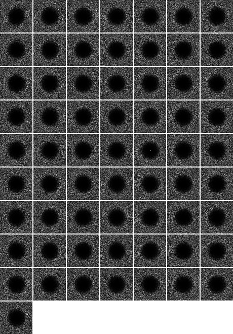
GetVoidAndClusterBlueNoise((64,64,64),(1.9,1.9,0.0)) using the same format for display as Figure 2. Note that all slices have the same properties.At first, it seems that this is exactly what we needed. Summing the Fourier transform along the third dimension now gives the desired 2D blue noise frequency distribution. Though, if you think about the meaning of this choice of parameters, you realize that it defeats the purpose of using 3D blue noise entirely. Having a standard deviation of zero along the third dimension means that the Gaussian filter blurs the slices of the volume independently. Thus, we are just computing independent 2D blue noise textures but at a much higher cost and without the strong guarantee on uniformity.
There is no sweet spot between these two extremes either. As soon as we increase the standard deviation sufficiently to get a useful exchange of information across slices, we get low-frequency components that are strong enough to cause problems. We have to conclude that we can only get arrays of high-quality 2D blue noise textures by computing them as independent 2D blue noise textures with independent random numbers. Any 3D blue noise texture with the characteristic properties in the frequency domain will necessarily have poor 2D blue noise properties.
Dithering with 3D blue noise
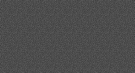
Now you may think that our initial motivation remains valid. The human visual system blurs in space and in time so 3D blue noise should still be good. This sounds convincing enough to give it a try. Figure 8 shows dithering with a 3D blue noise texture whereas Figure 9 shows dithering with independently computed 2D blue noise textures. Clearly, the 2D blue noise gives better results.


I am not a specialist on perception but the following explanation seems plausible to me. Humans are actually very sensitive to movement. Saying that the human visual system blurs in time is just wrong, at least for a 20 or 60 Hz refresh rate. If clusters of bright or dark pixels shift around, this is a movement that is very noticeable. Besides, the low-frequency components in the 3D blue noise make the tiling very obvious.
If you have spatially high-frequent 2D blue noise that changes in an uncorrelated fashion over time, there is not much of a movement to notice, so here the blurring over time works better. For comparison Figure 10 shows a single frame from Figure 9. It looks less uniform than Figure 9.
Valid applications of 3D blue noise
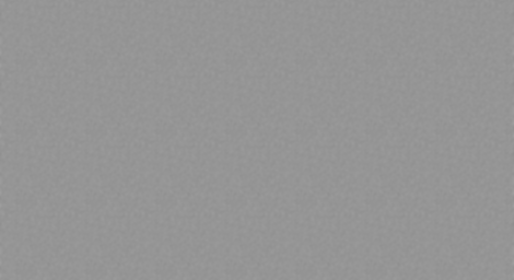
This does not mean that 3D blue noise is entirely useless. Basically, it is applicable whenever you really do blur over a 3D domain. Say for example that you are using 3D blue noise to accelerate a computation that fills a 3D volume texture. If you subsequently blur this volume texture over all three dimensions, the high-frequent components of the 3D blue noise vanish and you get a good approximation of the true continuous signal as shown in Figure 11. This result is significantly more uniform than the result obtained with independent 2D blue noise textures shown in Figure 12.

We may also rely on the human visual system to blur in the two spatial dimensions but apply an explicit blur in the third dimension. This scenario can arise when you do Monte Carlo integration. To do so you need multiple random numbers per pixel. You use each of them to evaluate some function and then take the mean of the results to get an estimate for the integral of the function. This is the basis of path tracing and many other methods in computer graphics.
Figure 13 and Figure 14 give you an idea of how that works. For the sake of this example, the function being integrated is just a unit-step function which basically means that we are still doing dithering. With 3D blue noise we get notably fewer extreme values (0.71% vs. 1.35% black pixels) and a lower standard deviation (0.120 vs. 0.133). At the same time the averaging is a box filter, which diminishes the high-frequent components along the third dimension. Thus, the 3D blue noise gains better 2D blue noise properties and tiling is no longer a problem. 3D blue noise may reduce variance in Monte Carlo integration. On the other hand, you have to be cautious because such a correlation between random numbers can introduce a bias into your estimation.

A database of 3D and 4D blue noise textures
As for 2D blue noise textures I have prepared a database of 3D and 4D blue noise textures that is available to download for free and dedicated to the public domain. Again this database includes, single-channel, two-channel, three-channel and four-channel textures where the channels are computed independently.
As a novelty, textures are also provided in a custom raw-data format now. This has the advantage that there are no rounding errors when storing textures with more than \(2^{16}\) different values. For 4D textures this is the only available format. A detailed description of this format is provided as part of the download. The database provides 3D blue noise textures with resolution 16³, 32³ and 64³ as well as 4D blue noise textures with resolution \(8^4\) and \(16^4\).
Conclusions
If 2D blue noise is what you want, then 2D blue noise is what you should use. Using 3D blue noise really only makes sense, if you explicitly blur along the third dimension. This precludes many tempting screen-space applications such as dithering and jittering. Still, there are challenges that call for 3D or even 4D blue noise. If you ever face them, the required blue noise textures are at your fingertips now.
References
R. A. Ulichney (1993). Void-and-cluster method for dither array generation. Proc. SPIE 1913, Human Vision, Visual Processing, and Digital Display IV. Official version | Author's version
Downloads
Comments
Patapom
2017-02-01, 22:25
Great analysis, thanks!
Won
2017-02-03, 19:07
Someone should check my handwaving, but I think you can get this result very quickly with the Fourier slice theorem.
Basically, projecting-then-fourier is equivalent to fourier-then-slicing. There is kind of a duality there, like convolution-then-fourier is equivalent to fourier-then-multiplication.
So what is the fourier transform of a 2-D slice of a volumetric blue noise texture? I believe the above tells you that it is the projection of the fourier transform of the volume (a solid with a ball bunched out), which is not going to be what you want (a plane with a disc punched out). Parts outside the sphere are going to land in the disc.
Christoph
2017-02-03, 23:02
Hi Won,
you are absolutely right, the Fourier slice theorem is equivalent to what I proved here. I never knew the statement under this name but it’s handy. Nonetheless, it’s nice to give the proof, especially if it’s just three steps plus the definition of the Fourier transform.
You are also right about the structure of the Fourier transform of the 2D slice. What you get is the sum of the slices in Figure 2 and that amounts to Figure 5.
Won
2017-02-16, 17:15
If you want to link me, I’m @won3d on twitter
Christoph
2017-02-17, 11:57
Done.
Cassidy Curtis
2017-03-14, 23:11
Wouldn’t a similar issue come up with 1D slices of a 2D blue noise texture? (I’ve been playing with your 2D noise textures, and misusing them in all kinds of horrible ways. Lots of nice artifacts have come up in the process, and it seems a subset of them could be explained this way.)
Anyway, thanks for the analysis, this is great stuff!
Christoph
2017-03-15, 1:23
Yes, absolutely. If you sum over the rows of the 2D Fourier transform shown in Figure 6, you get the 1D Fourier transform of a 1D column from the blue noise texture. The blue noise properties will be fairly poor, low frequency components would be only slightly weaker than higher frequencies.
If you want, you can use my code to generate 1D blue noise that actually has good blue noise properties. Just pass (1024,) as OutputShape where 1024 may be replaced by any other number of samples.
Cassidy Curtis
2017-03-16, 1:03
Fantastic, that works beautifully!
For the RGBA examples you created, were those 3D textures 4 pixels deep? Or is each channel a separate 2D texture with a different random seed?
Christoph
2017-03-16, 1:16
Neat. If you get the chance, you should store it into a *.wav file to get a feeling for the true meaning of high-frequent noise 😉 .
The RGBA textures are just four independently computed noise textures in one file. In nearly all scenarios this should be what you want. Even with a small number of slices the problem described above becomes relevant. It is only slightly weaker because with few samples you miss most of the exterior of the spherical center region.
Nah
2018-02-27, 3:30
Cook and DeRose discuss the slicing with respect to wavelet noise in their paper too.
https://graphics.pixar.com/library/WaveletNoise/paper.pdf
Joe Eagar
2018-04-20, 7:24
For blue noise masks in 3D I’ve found it more useful to use poisson dart throwing than void cluster, since you can do the poisson test in both 3d and in 2D along all three axes. It’s kind of slow though, thus is an ongoing area of research I think.
Christoph
2018-04-20, 11:13
I would be curious to see what the spectrum looks like that you get out of this approach. The point of what I wrote above is that any dither array with the typical 3D blue noise spectrum will have a poor 2D blue noise spectrum for its slices. There might be a tiny wiggle room though, since the Fourier coefficients are complex. If you are lucky, they might cancel out in just the right way but it would be surprising to me if this can be accomplished for all slices simultaneously.
Joe Eagar
2018-04-21, 7:32
Here’s the paper I went off of. It’s not terribly complicated.
http://resources.mpi-inf.mpg.de/ProjectiveBlueNoise/
I used it to generate a progressive sampling mask (like void-cluster), which is a bit of a pain with dart throwing. I think I only managed to generate a relatively small mask, but it was sufficient for my purposes.
Christoph
2018-04-21, 12:51
The focus in this paper is different from what I am discussing in this blog post. They generate blue noise point sets and consider their projection onto lower-dimensional subspaces (i.e. discarding a coordinate of each point) whereas I consider blue noise dither arrays and look at one 2D slice at a time. It is entirely plausible to me that you can construct 3D blue noise point sets with good 2D blue noise properties for some projections and that is certainly useful but the use cases for such point sets are different from use cases of dither arrays.
The equivalent of taking a slice out of a 3D blue noise dither array for a point set would be to only consider points with z-coordinates in some small interval and to project these points down to the xy-plane. For a sufficiently small z-interval, that should lead to issues that are very similar to those discussed in the blog post.
Joe Eagar
2018-04-21, 18:20
I did generate a dither array, for which I modified the method a bit. It was a pretty small mask though (16x16x16 or 32x32x32 I think), and took forever to generate. You’re right that it’s not perfect, but it was a lot better than just straight 3D blue noise.
That said, I used it for a pretty basic stochastic optimization problem at work. I’ve not tested how well it’d work for remeshing or any other sort of stress test.
Christoph
2018-04-23, 2:07
In that case I would still be curious to see the discrete Fourier transform of your dither array 🙂 .
Joe Eagar
2018-04-26, 1:14
I remember it took forever to generate the dither array. In the spirit of procrastination I’ve instead come up with a way to optimize the FFT of a dither mask directly. It’s kindof crude, but is useful enough. I’ve written a blog post on it:
thegraphicsblog.com/2018/04/25/controlling-noise-spectrum/
IIRC, the original FFT optimization method (whose patent recently expired I believe) was a lot better, but also somewhat more complicated.
Comments are closed.