Finding Real Polynomial Roots on GPUs
A recent paper of mine performs an intersection test in a ray tracing shader. To this end, I had to compute all real roots of a polynomial of moderately high degree (10 to 26). Overall, computing polynomial roots is an extremely well-studied problem where many highly accurate and reliable methods are available [Press2007]. However, implementations of such methods on GPUs are rarely found. After experimenting a bit with different options, I ended up implementing a recent polynomial solver proposed by Cem Yuksel [Yuksel2022]. I wrote my implementation from scratch in GLSL. A naive implementation has many nested loops or recursions and accesses arrays using loop counters. That is a recipe for register spilling, which is devastating to the performance of the shader. After a bit of puzzling, I ended up with an implementation that avoids this problem entirely. You can take a look at my implementation on Shadertoy and read on to learn more about how it works, why register spilling is an issue and how I resolved it.
Laguerre's method
Initially, I had concerns about Cem Yuksel's solver [Yuksel2022]. It is essentially a bracketed Newton bisection (see below). And Newton's method has a known failure case: It is bad at finding double roots such as the one in the polynomial \(x^2\). Basically, whenever the function does not change its sign at the root, Newton's method will struggle. It may diverge completely. For ray intersection tests, that happens at the silhouette of the shape being ray traced (see Figure 1). In the end, this was less of a problem than I had thought. With its bracketing and bisection, the solver has enough safeguards to still perform well when Newton's method itself does not.

At first, I was looking for other solutions. For cubic and quartic polynomials I had previously worked with closed-form solutions, but for polynomials of degree five or more that is simply impossible [Abel1826]. The solution must be iterative. The book Numerical Recipes [Press2007] is a treasure chest for numerical algorithms like that. Chapter 9.5 describes a variant of Laguerre's method, which provides a reliable way to find all roots of a polynomial (including complex roots). The overall procedure is to iterate towards a root \(x_0\), then divide the polynomial by \(x-x_0\) such that it no longer has this root and then find the next root. The way it works, the very first root that is found may already be a complex root, even when there are plenty of real roots to be found. After that, the polynomial will have complex coefficients. So basically, all arithmetic in this algorithm has to deal with complex numbers.
Porting the C++ code for Laguerre's method to GLSL was simple enough and overall, this method worked quite well. There were a few stability issues though. Sometimes, real roots would have a small imaginary part due to rounding errors. Telling real roots from complex roots was difficult at times. And for roots with multiplicity four or higher, which tends to happen at the center of my spherical harmonics glyphs, accuracy of all roots could suffer. It should be noted that my implementation used single-precision floats.
The bigger problem was that this method was not fast enough. My baseline was a ray marching procedure with a few clever optimizations [vanAlmsick2011]. Computing roots of a degree-10 polynomial ended up being more expensive than 100 ray marching steps with this method. The quality with 100 steps was not great but decent. So either the polynomial solver has to become faster or the method is not that appealing. Two aspects hamper its efficiency. Firstly, it has to compute all roots, including complex roots, to be sure that it has found all real roots. But the complex roots are simply discarded, so this work is wasteful. Secondly, all arithmetic is complex even though the original polynomial is real. Evaluating a complex polynomial at a complex point takes four times more instructions than evaluating a real polynomial at a real point. That factor hurts performance quite a bit. I ended up implementing bracketed Newton bisection [Yuksel2022] after all. In my measurements with degree-10 polynomials that was ca. 2.7 times faster. I will still keep Laguerre's method in mind for cases where I actually need complex roots.
Bracketed Newton bisection
I like to call Cem Yuksel's method bracketed Newton bisection, because it is an apt descriptive name. The original paper does not really name its technique [Yuksel2022]. What follows, is a brief summary of this method but of course the paper has more details. Say we have a polynomial of degree \(d\)
\[p(x)=a_dx^d + \ldots + a_2x^2 + a_1x + a_0\]with real coefficients \(a_0,\ldots,a_d\in\mathbb{R}\). We want to find all of its real roots, i.e. all numbers \(x\in\mathbb{R}\) such that \(p(x)=0\). If we have an interval \([a,b]\) such that \(p(a)p(b)\le0\), there must be a real root somewhere within this interval. Such an interval is called a bracket [Press2007]. Then bisection is one way to find a root: We evaluate \(p(\frac{a+b}{2})\). If that has the same sign as \(p(a)\), we set \(a\) to \(\frac{a+b}{2}\), otherwise we set \(b\) to \(\frac{a+b}{2}\). This way, the length of the interval is halved in each iteration but the interval always remains a bracket around a root. Once it is small enough, we have found the root with the desired accuracy.
Bisection is reliable but slow. It takes one iteration per binary digit of the root. For full accuracy with single-precision floats that would be ca. 23 iterations. Newton's method has rather complimentary strengths ([Press2007] chapter 9.4). It is fast but unreliable. The idea is to start with some guess \(x_0\in\mathbb{R}\) for the root. Then the derivative is used to construct a tangent line to the graph of \(p(x)\) at \(x_0\). The root of this tangent line is used as approximation of the root. It is
\[x_{n+1}=x_{n} - \frac{p(x_n)}{p^\prime (x_n)}\text{.}\]If the initialization is close enough to the root, this method converges quadratically. That means that the number of correct digits in the root will double with each iteration. Over the course of three iterations, you might go from 1 to 2, to 4, to 8 correct digits. This exponential growth in the number of correct digits is much faster than the linear growth with bisection. The downside is that the method may end up walking in circles when the initialization is not good enough and that it struggles with double roots. At a double root, \(p^\prime(x)=0\). For a point near that double root, Newton's method divides by a small number, which may lead to \(x_{n+1}\) being much farther from the root than \(x_n\).
Therefore, Newton bisection combines both methods, trying to harvest the strengths of both. In each iteration, it maintains an interval \([a_n,b_n]\) and a current guess for the root \(x_n\). The first guess is \(x_0=\frac{a_0+b_0}{2}\). Depending on the sign of \(p(x_n)\), either \(a_{n+1}\) or \(b_{n+1}\) is set to \(x_n\), while the other interval end remains unchanged. If Newton's method produces an \(x_{n+1}\) outside of the interval \([a_{n+1},b_{n+1}]\), that result will be rejected and \(x_{n+1}\) is set to \(\frac{1}{2}(a_{n+1}+b_{n+1})\) instead. Otherwise, Newton's method runs undisturbed.
Now we have a reliable way to find a single root inside a bracket. If there are multiple real roots in a bracket, we will only find one of them. Since our goal is to find all real roots, we need to find brackets containing exactly one root. We can be sure of that if the polynomial \(p(x)\) is either monotonically increasing or decreasing within the bracket. The polynomial is monotonic between two roots of its derivative \(p^\prime(x)\) and to the left/right of the first/last root of \(p^\prime(x)\). Thus, we can first find all real roots of \(p^\prime(x)\) and then the intervals defined by these roots where the signs of \(p(x)\) at the end points differ each contain exactly one real root. To find roots of \(p^\prime(x)\), we repeat this method recursively, moving to derivatives of ever-increasing order. Eventually, we reach a derivative of degree 2 and can compute both of its roots using the quadratic formula. With that, we have a method that is guaranteed to find all real roots in a given interval.
There are a few more aspects to Cem Yuksel's solver that I will not discuss in any detail here and have not implemented [Yuksel2022]. For example, there is a specialized version for cubic polynomials and a variant that does not require a bracket around all real roots as input. Please take a look at the paper if you are interested.
Keeping track of brackets
The way it is phrased above, bracketed Newton bisection should be implemented in a recursive fashion: The method to compute roots of a polynomial \(p(x)\) of degree \(d\) invokes the method to compute roots of a polynomial \(p^\prime(x)\) of degree \(d-1\). Indeed, this is how Cem Yuksel's C++ implementation does it. Though, when writing shaders I am wary of recursion. For one thing, recursion is explicitly prohibited in WebGL and I wanted to put my implementation on Shadertoy. Besides, the compiler stack for GLSL relies on inlining extensively and I am worried that a recursive implementation would generate poorly optimized code.
Instead, we could allocate a 2D array to store the roots of \(p(x)\) and all of its derivatives. A polynomial of degree \(d\) has at most \(d\) real roots, so a \(d\times(d-1)\) array would certainly be big enough. The derivative of \(p(x)\) is
\[p^\prime(x) = \sum_{j=0}^{d-1} (j+1)a_{j+1}x^j\text{.}\]Applying this formula iteratively, we find that the \(k\)-th derivative of \(p(x)\) is
\[p^{(k)}(x) = \sum_{j=0}^{d-k} \frac{(j+k)!}{j!} a_{j+k}x^j\text{.}\]Thus, we can easily get the coefficients of the quadratic derivative \(p^{(d-2)}(x)\) without computing all the other derivatives recursively. Then we compute its roots, and put them into our 2D array. After that, we start a loop to compute roots for derivatives of increasing degree, using the roots computed in the previous iteration.
This 2D array is pretty big though. If the compiler were to decide to allocate one register for each of its entries, the register pressure would be immense. Probably the compiler is clever enough to avoid that, but it is safer to avoid the issue altogether. My implementation only uses a single array of roots with \(d+1\) entries (i.e. one more than needed for \(p(x)\)). The user provides a bracket \([a,b]\) around all sought-after roots. Initially, all entries are set to \(a\), except for the last one which is set to b. Then roots of the \(k\)-th derivative are stored in entries \(k\) to \(d-1\), i.e. in the back of the array. With this pattern, roots are overwritten just after they were needed for the last time.
This pattern has a couple of advantages. Overall, the index arithmetic is simple and the code is quite readable. In each iteration, the relevant brackets are simply all pairs of two consecutive entries in the array because we compute roots in sequence and we put \(a\) and \(b\) at the beginning and end of the array. We can set two consecutive entries to identical values to indicate that a bracket should be skipped. This is useful when the \(k\)-th derivative has less than \(d-k\) roots. Then it is also safe to always iterate over all brackets. Brackets of the form \([a,a]\) that are left over from the initialization of the array will be skipped. We can use the exact same code without any specialization for all the different derivatives. And for reasons that I explain below, that is actually a good idea.
Once we have computed roots for \(p(x)\), they are immediately in a format that is suitable as end result of the algorithm. The only difference is that we write a special value called NO_INTERSECTION into the array when a bracket does not contain a root (instead of producing an empty bracket).
Register spilling
The reasons I alluded to above are related to register spilling and unrolling. Avoiding spills was one of the major goals with this implementation. There are a couple of rules to follow to avoid spills, so before I go any further, I want to explain what register spilling is, why it is best to avoid it and how that can be done.
What is a register anyway? GPUs have various kinds of memory. The most well-known kind is VRAM. On modern consumer GPUs you get something like 8 to 16 GB of VRAM with a bandwidth in the ballpark of 500 GB/s. In addition, GPUs have several levels of cache, which I will call L1, L2 and L3. Current NVIDIA GPUs do not have an L3 cache but AMD GPUs do. Intel uses different names, but I will stick to NVIDIA terminology here. Before the compute units get to do anything with data from VRAM, it goes through the cache hierarchy. If it happens to be already there from a previous transaction (i.e. it is cached), there is no need to read it from VRAM again. L1 is the fastest and smallest cache. But GPUs have an even faster kind of memory: The register file. Registers provide the inputs and outputs for arithmetic instructions. If my math is right, an RTX 4070 has a total space of
\[46\cdot4\cdot16384\cdot4 \text{ B} = 11.5\text{ MiB} = 12.06\text{ MB}\]for registers across all of its streaming multiprocessors (SMs). And without boost it has 22.61 TFLOPS in single-precision arithmetic. If each of these instructions is an fma, which reads three floats from registers and writes one float, we get a total peak bandwidth for the register files of
\[\frac{22.61\text{ T}}{\text{s}}\cdot(3+1)\cdot4\text{ B} = 362\,\frac{\text{TB}}{\text{s}}\text{.}\]That is 718 times more than the VRAM bandwidth. It is needless to say then, that it is desirable to ensure that instructions work with registers directly, rather than fetching their inputs from the memory hierarchy.
When threads are launched on a GPU, they are assigned a set of registers from the register file. Each instruction of the machine code executed by these threads holds hard-coded indices for registers in this set. With that in mind, consider the following piece of code as a problematic example. It is not related to polynomials but instead aims to extract positive numbers from an array:
int numbers[6] = { 2, -3, 5, 7, -1, -2 };
int positive_count = 0;
for (int i = 0; i != 6; ++i) {
    if (numbers[i] > 0) {
        numbers[positive_count] = numbers[i];
        positive_count++;
    }
}
In the end, positive_count will be 3 and the first three entries of numbers will be 2, 5 and 7. With this particular code, the entries of numbers are hard-coded and the whole loop would be optimized away. But if numbers were loaded from some buffer, this code would be a sure-fire way to cause register spilling.
The culprit is the expression numbers[positive_count]. It accesses an entry of an array using the index positive_count. The value of this index depends on the computations performed thus far. Depending on how many of the array entries were positive, different entries of the array will be accessed. If the array were stored in registers, there would be no way to hard-code the indices in the machine code. Therefore, this array will not be stored in registers. It will spill, which means that it is stored somewhere in the cache hierarchy. NVIDIA calls this concept local memory. Then the compute units are able to access array entries with dynamically computed indices, so the code will work as expected. But every interaction with the array now has to read memory from the caches. It may be L1, L2, L3 or even VRAM, depending on whether the data got evicted from the faster caches. The overhead of reading from L1 is moderate, but beyond this point, the reads and writes will be considerably slower than fetching the value from a register. And either way, these loads and writes are additional instructions that take time to execute.
When I profile shaders, register spilling is a common reason why they perform worse than expected. Eliminating spilling can give huge speedups. You can find timings below. With growing complexity of shaders (and the underlying compiler infrastructure), it can become tricky to avoid spills. In some cases, they may be the lesser of two evils, but at least with compute-intensive code I have never found a reason to tolerate spilling thus far.
To learn how to avoid spills, let us look at another example:
int numbers[6] = { 2, -3, 5, 7, -1, -2 };
int sum = 0;
for (int i = 0; i != 6; ++i)
    sum += numbers[i];
Does this code cause spilling (if it were not optimized away)? That depends on whether or not the index i qualifies as compile-time constant. If the loop is really implemented as a loop, where the index i is increased after each iteration, the index is the result of a computation. It is not known at compile time and cannot be hard-coded into the machine code. Then this code really causes spilling. To avoid that, we could rewrite the code snippet as follows:
int numbers[6] = { 2, -3, 5, 7, -1, -2 };
int sum = 0;
sum += numbers[0];
sum += numbers[1];
sum += numbers[2];
sum += numbers[3];
sum += numbers[4];
sum += numbers[5];
We have turned each iteration through the loop into separate instructions and in doing so we have hard-coded the indices. That circumvents the problem but is not pretty to look at. Thankfully, we can let the GLSL compiler do it for us:
int numbers[6] = { 2, -3, 5, 7, -1, -2 };
int sum = 0;
[[unroll]]
for (int i = 0; i != 6; ++i)
    sum += numbers[i];
By using the [[unroll]] directive, we have asked the compiler to copy the loop body once per iteration. This directive requires the GL_EXT_control_flow_attributes GLSL extension to be enabled. Of course, that is only possible when the number of iterations is known in advance. It is also not guaranteed that the compiler will take the hint. In the context of ray tracing, I encountered a case where it did not. That motivated me to resort to a less elegant solution (sorry).
Of course, for a summation like the one above, it would be better to simply sum up all the values as they are loaded from memory. Then there is no need for dynamic indexing or unrolling. In general, unrolling is a mighty weapon against register spilling but it is not without drawbacks. It is not always applicable and it inflates the machine code considerably, which can be a problem in itself. For one thing, more code usually means longer compile times. And for another, code also has to find its way from VRAM to a special cache (the instruction cache). The more code you have, the more likely it is that the code you would like to execute is not readily available from the instruction cache. Eventually that results in more cycles spent without issuing an instruction and thus lower efficiency. My rule of thumb is to unroll where I cannot avoid register spilling without it and to loop otherwise (using the [[loop]] directive).
Bracketed Newton bisection without spills
Now let us go back to the problem at hand: Implementing bracketed Newton bisection. The Newton bisection itself is not hard to implement for a polynomial with known coefficients. Horner's method helps to evaluate the polynomial and its derivative ([Press2007] p. 202). Loops over polynomial exponents are unrolled. Once we have it, the Newton bisection is invoked in a double loop. The outer loop works its way to derivatives of decreasing order \(k\). This loop is not unrolled in my implementation because it is not strictly necessary to avoid spilling and did not reduce the run time. As a consequence, unrolling polynomial evaluation for degree \(d-k\) instead of degree \(d\) is not an option. That is slightly wasteful but the best middle ground I could find. The inner loop iterates over the brackets in the array of roots described above. This one has to be unrolled because the loop index determines which array entries are dealt with.
Before we can actually invoke Newton bisection, we need the coefficients \(b_0,\ldots,b_{d-k}\) of the polynomial derivative
\[p^{(k)}(x) = \sum_{j=0}^{d-k} b_jx^j = \sum_{j=0}^{d-k} \frac{(j+k)!}{j!} a_{j+k}x^j\text{.}\]Their computation turned out to be one of the harder puzzles in this implementation. The naive solution is to simply set
\[b_j = \frac{(j+k)!}{j!} a_{j+k}\]but there are two problems with that. Firstly, I decided not to unroll with respect to \(k\), so the array access for \(a_{j+k}\) will cause spilling. Secondly, we need the factorials. Computing them using a loop every time we need such a coefficient is costly. We could precompute a table of factorials but then the array access will cause memory reads again.
After a bit of puzzling, I ended up with the following solution. All I care about are the roots of \(p^{(k)}(x)\), so there is no harm in scaling this function by some non-zero factor. I chose to compute the coefficients of \(\frac{1}{k!} p^{(k)}(x)\). These coefficients are
\[\frac{b_j}{k!} = \frac{(j+k)!}{j!k!} a_{j+k} = \frac{(j+k)!}{k!(j+k-k)!} a_{j+k} = \binom{j+k}{k} a_{j+k}\text{.}\]I am using a binomial coefficient here as shorthand for all these factorials. The nice thing about this reformulation is that the coefficient \(\frac{b_0}{k!}\) is simply \(\binom{k}{0} a_k = a_k\). Thus, it can be copied directly from the original polynomial. We can just loop over all coefficients once and copy the one that we want, like this:
[[unroll]]
for (int i = 0; i != MAX_DEGREE - 2; ++i)
    derivative[0] = (degree == MAX_DEGREE-i)
                  ? poly[i] : derivative[0];
But what about all the other coefficients? Recall that we do all of this for derivatives of decreasing order (i.e. increasing degree). After working with the derivative \(p^{(k+1)}(x)\), we need \(p^{(k)}(x)\). The opposite of taking a derivative is integration and integrals of polynomials are easy to compute. The integral of \(x^j\) is \(\frac{x^{j+1}}{j+1} + C\). The \(+C\) term is the constant coefficient that we already dealt with. Other than that, we just shift all the coefficients one place to the right and multiply by \(\frac{k+1}{j+1}\).
With these tricks, we have arrived at an implementation that avoids spilling reliably. Whenever a loop counter is used as index, this loop is unrolled. The outermost loop, which iterates over the order of the derivative \(k\), and the loop that iterates over iterations of Newton bisection are not unrolled. They do not need it because they perform exactly the same work on different values in each iteration. They are annotated with [[loop]].
Profiling and timings
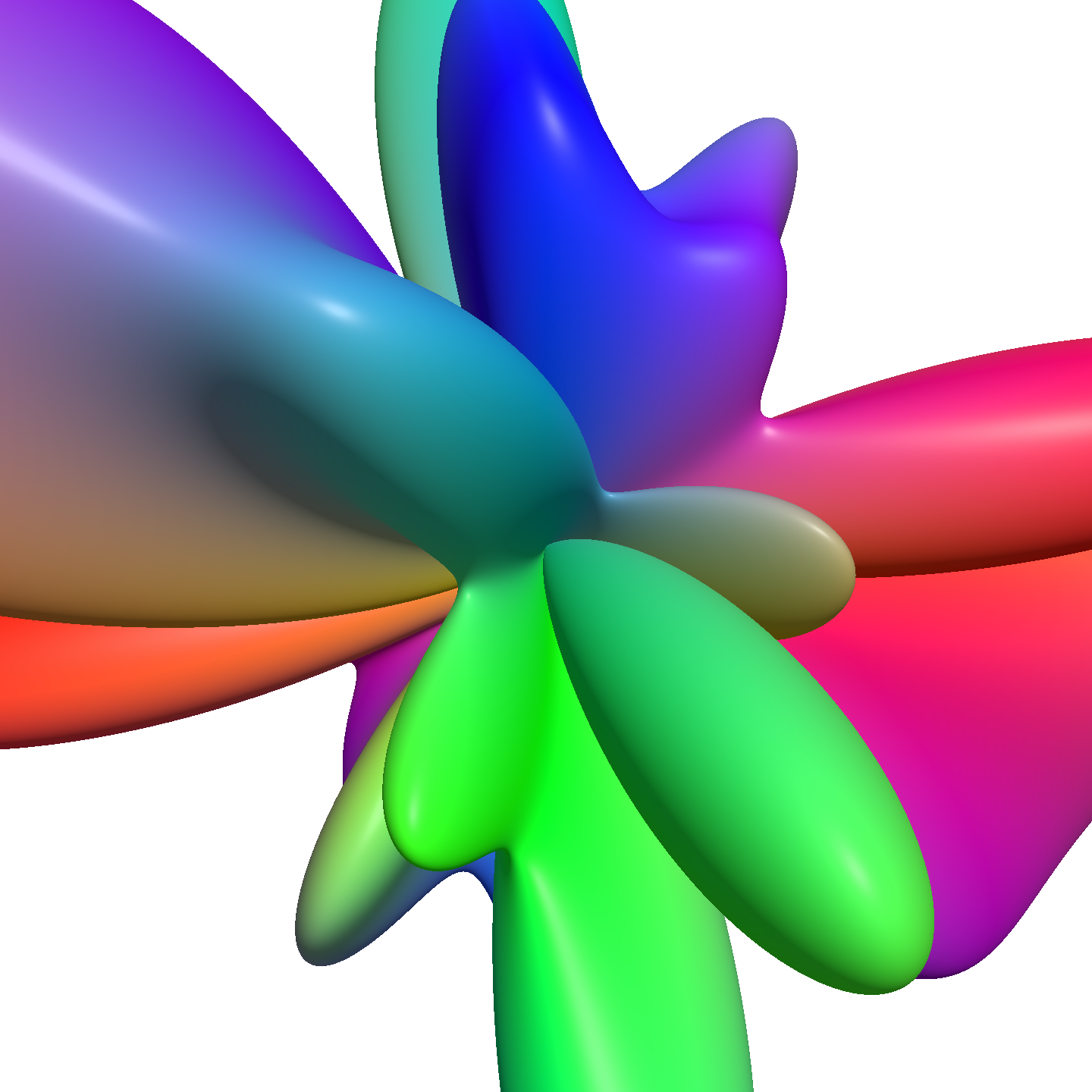
Above I have conveyed my mental model regarding register spilling. I hope that it will be useful to others but it is important to emphasize that all decisions about performance should be underpinned by profiling. Do not just assume that you know what the compiler stack will do for a particular shader and where the bottlenecks will be in the hardware. I have the most experience with NVIDIA Nsight Graphics but each hardware platform has suitable profiling tools. To substantiate my reasoning above, this section presents frame times and profiling results. All of them are measured on an NVIDIA RTX 2070 Super. The benchmark is to render Figure 2 using my Shadertoy. I ran the Shadertoy offline in an environment where GL_EXT_control_flow_attributes is available.

zoom=1.2 and iTime=0.0 in the Shadertoy.To investigate the impact of register spilling, consider the following alternative code for derivative computation:
float factorial[19] = { 1.0, 1.0, 2.0, 6.0, 24.0, 120.0, 720.0, 5040.0, 40320.0, 362880.0, 3628800.0, 39916800.0, 479001600.0, 6227020800.0, 87178291200.0, 1307674368000.0, 20922789888000.0, 355687428096000.0, 6402373705728000.0 };
int k = MAX_DEGREE - degree;
for (int j = 0; j != degree + 1; ++j)
    derivative[j] = factorial[j + k]
        / factorial[j] * poly[j + k];
In the previous section, we concluded that it is a bad idea to use this approach. Accessing factorial[j+k] and poly[j+k] will cause spilling. Indeed the Nsight throughput metrics in Figure 3 reveal issues. With 45.8%, the SM throughput is not that high. The SMs are where the compute units are, so we would expect high throughput in such a compute-heavy shader. However, the L2 cache has a throughput of 11.7%, which is unexpected in a shader that does not explicitly read/write anything from/to VRAM. This is a telltale sign of register spilling. Depending on your profiling tools, you may have access to metrics that reveal spilling more directly. The keyword to look out for on NVIDIA hardware is local memory.

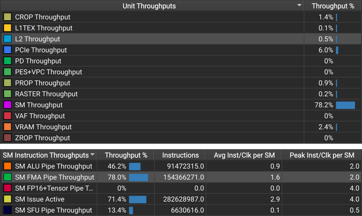
Looking at the metrics for my optimized implementation in Figure 4, we see a different picture. L2 throughput is low, SM throughput is high and the FMA pipe has a throughput of 78%. This throughput is satisfactory. The FMA pipe is what should be the bottleneck here, since the innermost loop evaluates polynomials using Horner's method. And a throughput significantly above 80% is always hard to achieve. At this point, the next meaningful optimization is to reduce the number of fused-multiply-add instructions needed by the algorithm. That could potentially be done by specializing the bracketed Newton bisection to the lower degrees of the various derivatives. But I could not get the compiler to do that for me without introducing issues that were more detrimental to the overall run time.
It is also insightful to look at some absolute numbers. All timings in the following table are frame times for rendering Figure 2. The last one is the root finding implementation in my Shadertoy. The first one uses the bad derivative computation in the code listing above. It is 3.3 times slower, so it has been clearly worthwhile to put some thought into this. Additionally, the table explores a few variants regarding the use of [[unroll]] and [[loop]] directives. Removing [[loop]] directives makes no difference here, which indicates that my driver makes the same decisions as I. However, replacing both [[loop]] directives by [[unroll]] directives makes the shader much less efficient. That illustrates that too much unrolling can also be an issue. Removing [[unroll]] directives doubles the frame time, so the compiler really needed these hints to produce optimal code.
| Variant (all for degree 10) | Timing |
|---|---|
| With spilling derivative computation | 4.82 ms |
No [[unroll]] or [[loop]] directives | 2.99 ms |
No [[unroll]] directives | 2.99 ms |
[[loop]] directives replaced by [[unroll]] | 3.85 ms |
No [[loop]] directives | 1.46 ms |
| Optimized implementation | 1.46 ms |
The examples above use polynomials of degree 10. To see whether the implementation holds up for higher degree, let us consider an example with polynomials of degree 18 (Figure 5). That increases the frame time for the optimized implementation to 10.4 ms (7.1 times more). This increase is significant but based on the nesting of loops, we expect roughly cubic scaling here. Nsight reports 79.1% FMA pipe throughput, which is marginally better than for the lower degree. For the different variants of looping and unrolling, we get a similar picture as before. However, the derivative computation with spilling is a complete disaster here, taking 255 times longer than the optimized implementation. My best guess is that it spills all the way to VRAM.
| Variant (all for degree 18) | Timing |
|---|---|
| With spilling derivative computation | 2650 ms |
No [[unroll]] or [[loop]] directives | 25.9 ms |
No [[unroll]] directives | 25.9 ms |
[[loop]] directives replaced by [[unroll]] | 15.3 ms |
No [[loop]] directives | 10.4 ms |
| Optimized implementation | 10.4 ms |
SH_DEGREE, which is 8.As a final thought on timings, I want to convey a rough idea of how this GPU implementation performs in comparison to a CPU implementation. To this end, I will compare directly to the numbers reported by Cem Yuksel, which were measured on an “Intel Xeon CPU E5-2643 v3 at 3.4 GHz using single-threaded computation” [Yuksel2022]. For a degree-10 polynomial with lax error thresholds, the reported CPU timing is 1.45 µs. Comparing that to our timing shows a speedup factor of
\[\frac{1440^2}{1.46\text{ ms}}1.45\,\mathrm{\mu s} = 2059\text{.}\]Not bad, but take it with a grain of salt, please. The comparison is unfair for several reasons: The CPU implementation uses double-precision arithmetic and deals with a different set of polynomials, potentially with more real roots to be found. And it is not fair to compare a single thread to thousands of threads on a GPU. Also, the CPU is from 2014, whereas my GPU is from 2019. Nonetheless, this comparison illustrates that modern GPUs sport substantially more compute power than CPUs and that it is viable to put it to use on relevant problems.
Quality of roots
Speaking of double-precision arithmetic, I should say a few things about numerical stability of my implementation, which uses single-precision arithmetic only. For the spherical harmonics glyphs, the solver does not cause any obvious artifacts up to polynomials of degree 18 (see Figure 1). For degree 22 there are visible artifacts (see Figure 6) and for degree 26 they become quite objectionable (see Figure 7). I am using an error tolerance of \((b-a)10^{-4}\) but that can be adjusted on the first line of find_roots().


That is not to say, that you will always get the desired result when you use this solver to compute roots of a polynomial of degree less than 20. It depends heavily on how the roots of the polynomial are distributed ([Press2007] chap. 9.5) and how the polynomial coefficients are computed. When you have many roots with similar values far from zero (e.g. 1017, 1017.4 and 1018.1) any solver will struggle. The problem is that in this case small errors in the coefficients of the polynomial \(a_0,\ldots,a_d\) will lead to large errors in the roots. Even if the roots of the polynomial with the given coefficients were computed with infinite accuracy, the result would likely not be what you want because the input coefficients have rounding errors.
The easiest way to sidestep such issues is to put some thought into the choice of the coordinate frame. If you know that all roots are likely to be centered around a particular value of \(x\), you should shift coordinates such that this value becomes zero. That can make a huge difference in terms of stability. Section 3.3 of my paper discusses this approach in more detail and Cem Yuksel's paper provides further evaluations regarding stability [Yuksel2022].
Conclusions
There are two major takeaways here. Firstly, computing real roots of polynomials of moderately high degree (up to 20) in shaders is absolutely viable. Cem Yuksel's solver works well and my GPU implementation of it is reasonably optimized. There may be some headroom left for further optimization but for now, you are unlikely to find a faster method, at least with regard to the typical requirements of computer graphics applications. I have tested it on NVIDIA Turing and Intel Alchemist GPUs and got satisfactory timings. I think the reasoning behind my optimizations should age relatively well, but of course it makes sense to profile the code on newer/other architectures when you want to rely on it.
Secondly, this blog post is a neat case study of how register spilling can impact performance and how it can be avoided. In my experience, spilling is one of the most treacherous performance cliffs. An otherwise well-optimized shader may contain a single inconspicuous line of code that causes spilling and triples the run time. Avoiding spilling often requires some creativity. For example, in two of my past papers, I used sorting networks to do so. But outside of ray-tracing shaders (where the compiler does all sorts of things under the hood), I have never encountered a case where I was unable to avoid spills. And when I did so, that was usually the most worthwhile optimization.
References
Abel, Niels Henrik (1826). Beweis der Unmöglichkeit, algebraische Gleichungen von höheren Graden als dem vierten allgemein aufzulösen. Journal für die reine und angewandte Mathematik 1(1). Archive version | Official version
Press, William H. and Teukolsky, Saul A. and Vetterling, William T. and Flannery, Brian P. (2007). Numerical recipes: The art of scientific computing (third edition). Cambridge University Press. Author's version | Official version
van Almsick, Markus and Peeters, Tim H. J. M. and Prckovska, Vesna and Vilanova, Anna and ter Haar Romeny, Bart (2011). GPU-Based Ray-Casting of Spherical Functions Applied to High Angular Resolution Diffusion Imaging. IEEE TVCG 17(5). Author's version | Official version
Yuksel, Cem (2022). High-Performance Polynomial Root Finding for Graphics. Proceedings of the ACM on Computer Graphics and Interactive Techniques 5(3). Author's version | Official version
Code listing
Here is the full GLSL code for my implementation of bracketed Newton bisection [Yuksel2022]. With 151 lines of code, it is quite a bit shorter than the 1513-line C++ implementation by Cem Yuksel but it also implements less features. It makes use of [[unroll]] and [[loop]] directives extensively, so it requires GL_EXT_control_flow_attributes to be enabled. To use find_roots() you need to come up with some reasonably tight bracket \([a,b]\) for the location of the roots you are searching. If it is too big, that can increase the iteration count and thus the cost. If it is too small, you will simply not get the roots outside of the bracket but the roots that you get will be accurate nonetheless.
Porting this code to any other C-like language should be extremely simple. Just change the syntax of the two parameter lists, replace the [[unroll]] and [[loop]] directives by suitable constructs (e.g. #pragma) and make sure that mathematical functions such as sqrt(), abs() and clamp() are available. The code is licensed under a CC0 1.0 Universal License.
// The degree of the polynomials for which we compute roots
#define MAX_DEGREE 10
// When there are fewer intersections/roots than theoretically possible, some
// array entries are set to this value
#define NO_INTERSECTION 3.4e38


// Searches a single root of a polynomial within a given interval.
// \param out_root The location of the found root.
// \param out_end_value The value of the given polynomial at end.
// \param poly Coefficients of the polynomial for which a root should be found.
//        Coefficient poly[i] is multiplied by x^i.
// \param begin The beginning of an interval where the polynomial is monotonic.
// \param end The end of said interval.
// \param begin_value The value of the given polynomial at begin.
// \param error_tolerance The error tolerance for the returned root location.
//        Typically the error will be much lower but in theory it can be
//        bigger.
// \return true if a root was found, false if no root exists.
bool newton_bisection(out float out_root, out float out_end_value,
    float poly[MAX_DEGREE + 1], float begin, float end,
    float begin_value, float error_tolerance)
{
    if (begin == end) {
        out_end_value = begin_value;
        return false;
    }
    // Evaluate the polynomial at the end of the interval
    out_end_value = poly[MAX_DEGREE];
    [[unroll]]
    for (int i = MAX_DEGREE - 1; i != -1; --i)
        out_end_value = out_end_value * end + poly[i];
    // If the values at both ends have the same non-zero sign, there is no root
    if (begin_value * out_end_value > 0.0)
        return false;
    // Otherwise, we find the root iteratively using Newton bisection (with
    // bounded iteration count)
    float current = 0.5 * (begin + end);
    [[loop]]
    for (int i = 0; i != 90; ++i) {
        // Evaluate the polynomial and its derivative
        float value = poly[MAX_DEGREE] * current + poly[MAX_DEGREE - 1];
        float derivative = poly[MAX_DEGREE];
        [[unroll]]
        for (int j = MAX_DEGREE - 2; j != -1; --j) {
            derivative = derivative * current + value;
            value = value * current + poly[j];
        }
        // Shorten the interval
        bool right = begin_value * value > 0.0;
        begin = right ? current : begin;
        end = right ? end : current;
        // Apply Newton's method
        float guess = current - value / derivative;
        // Pick a guess
        float middle = 0.5 * (begin + end);
        float next = (guess >= begin && guess <= end) ? guess : middle;
        // Move along or terminate
        bool done = abs(next - current) < error_tolerance;
        current = next;
        if (done)
            break;
    }
    out_root = current;
    return true;
}


// Finds all roots of the given polynomial in the interval [begin, end] and
// writes them to out_roots. Some entries will be NO_INTERSECTION but other
// than that the array is sorted. The last entry is always NO_INTERSECTION.
void find_roots(out float out_roots[MAX_DEGREE + 1], float poly[MAX_DEGREE + 1], float begin, float end) {
    float tolerance = (end - begin) * 1.0e-4;
    // Construct the quadratic derivative of the polynomial. We divide each
    // derivative by the factorial of its order, such that the constant
    // coefficient can be copied directly from poly. That is a safeguard
    // against overflow and makes it easier to avoid spilling below. The
    // factors happen to be binomial coefficients then.
    float derivative[MAX_DEGREE + 1];
    derivative[0] = poly[MAX_DEGREE - 2];
    derivative[1] = float(MAX_DEGREE - 1) * poly[MAX_DEGREE - 1];
    derivative[2] = (0.5 * float((MAX_DEGREE - 1) * MAX_DEGREE)) * poly[MAX_DEGREE - 0];
    [[unroll]]
    for (int i = 3; i != MAX_DEGREE + 1; ++i)
        derivative[i] = 0.0;
    // Compute its two roots using the quadratic formula
    float discriminant = derivative[1] * derivative[1] - 4.0 * derivative[0] * derivative[2];
    if (discriminant >= 0.0) {
        float sqrt_discriminant = sqrt(discriminant);
        float scaled_root = derivative[1] + ((derivative[1] > 0.0) ? sqrt_discriminant : (-sqrt_discriminant));
        float root_0 = clamp(-2.0 * derivative[0] / scaled_root, begin, end);
        float root_1 = clamp(-0.5 * scaled_root / derivative[2], begin, end);
        out_roots[MAX_DEGREE - 2] = min(root_0, root_1);
        out_roots[MAX_DEGREE - 1] = max(root_0, root_1);
    }
    else {
        // Indicate that the cubic derivative has a single root
        out_roots[MAX_DEGREE - 2] = begin;
        out_roots[MAX_DEGREE - 1] = begin;
    }
    // The last entry in the root array is set to end to make it easier to
    // iterate over relevant intervals, all untouched roots are set to begin
    out_roots[MAX_DEGREE] = end;
    [[unroll]]
    for (int i = 0; i != MAX_DEGREE - 2; ++i)
        out_roots[i] = begin;
    // Work your way up to derivatives of higher degree until you reach the
    // polynomial itself. This implementation may seem peculiar: It always
    // treats the derivative as though it had degree MAX_DEGREE and it
    // constructs the derivatives in a contrived way. Changing that would
    // reduce the number of arithmetic instructions roughly by a factor of two.
    // However, it would also cause register spilling, which has a far more
    // negative impact on the overall run time. Profiling indicates that the
    // current implementation has no spilling whatsoever.
    [[loop]]
    for (int degree = 3; degree != MAX_DEGREE + 1; ++degree) {
        // Take the integral of the previous derivative (scaled such that the
        // constant coefficient can still be copied directly from poly)
        float prev_derivative_order = float(MAX_DEGREE + 1 - degree);
        [[unroll]]
        for (int i = MAX_DEGREE; i != 0; --i)
            derivative[i] = derivative[i - 1] * (prev_derivative_order * (1.0 / float(i)));
        // Copy the constant coefficient without causing spilling. This part
        // would be harder if the derivative were not scaled the way it is.
        [[unroll]]
        for (int i = 0; i != MAX_DEGREE - 2; ++i)
            derivative[0] = (degree == MAX_DEGREE - i) ? poly[i] : derivative[0];
        // Determine the value of this derivative at begin
        float begin_value = derivative[MAX_DEGREE];
        [[unroll]]
        for (int i = MAX_DEGREE - 1; i != -1; --i)
            begin_value = begin_value * begin + derivative[i];
        // Iterate over the intervals where roots may be found
        [[unroll]]
        for (int i = 0; i != MAX_DEGREE; ++i) {
            if (i < MAX_DEGREE - degree)
                continue;
            float current_begin = out_roots[i];
            float current_end = out_roots[i + 1];
            // Try to find a root
            float root;
            if (newton_bisection(root, begin_value, derivative, current_begin, current_end, begin_value, tolerance))
                out_roots[i] = root;
            else if (degree < MAX_DEGREE)
                // Create an empty interval for the next iteration
                out_roots[i] = out_roots[i - 1];
            else
                out_roots[i] = NO_INTERSECTION;
        }
    }
    // We no longer need this array entry
    out_roots[MAX_DEGREE] = NO_INTERSECTION;
}